Variational autoencoders
Variational autoencoders (VAEs) are probabilistic generative models that represent the joint distribution $p(x, z)$ of data $x$ and latent variables $z$. The latent variables control the data-generating process, but we cannot directly observe them. In VAEs, the evidence $p(x\vert \theta)$ is computed by marginalizing over the latent variables:
\[p(x \vert \phi) = \int p(x \vert z, \phi) p(z)dz\]This decomposition into the prior $p(x)$ and posterior $p(x\vert z, \phi)$ is powerful because even if both distributions are relatively simple, their combination can capture a complex data distribution $p(x \vert \phi)$. Typically, both are the multivariate Normal. For instance, $p(x) = \text{Norm}_x \big[0, I\big]$ and $p(x \vert z, \phi) = \text{Norm}_x \big[\mu, \sigma^2I\big]$ where the mean $\mu$ is predicted by a neural network $f(z, \phi)$, representing the important aspects of data, while $\sigma I$ accounts for the noise, the remaining unexplainable variation.
\[\gray p(x \vert \phi) = \int \Norm \mu {\sigma^2 I}\Norm 0 I dz\]This can be viewed as an infinite mixture of Gaussians with different means. To train the network, we aim to maximize the log-likelihood:
\[\hat\phi = \argmax \phi \Big[\sum_i \log p(x_i \vert \phi)\Big]\]The problem is that there is no closed-form expression for the above integral, making it intractable. Moreover, Monte Carlo estimation fails because $p(z)$ often assigns probability to regions where the likelihood $p(x \vert z, \phi)$ is negligible, thus contributing little to the integral, leading to unstable estimates.
Deriving the lower bound
Although the integral still remains intractable, we introduce an arbitrary distribution over the latent variables $q(z \vert \phi)$ to focus on regions where $p(x\vert z, \phi)$ is high, enabling Monte Carlo estimation. We can then derive the integral lower bound using Jensen’s inequality (proved in the appendix), which states that for a concave function $g$:
\[\gray g(EX) \ge E\big[ g(x)\big]\]Since we are maximizing the log-likelihood and the logarithm is concave, we can derive the Evidence Lower Bound (ELBO):
\[\log p(x \vert \phi) = \log \Big[\int q(z \vert \theta) \frac {p(x, z \vert \phi)}{q(z \vert \phi)} dz\Big] \ge \int q(z\vert \theta) \log \Big[ \frac{p(x, z \vert \phi)}{q(z\vert \theta)}\Big] dz \gray = \text{ELBO}\big[\theta, \phi \big]\]Simplify the right hand side, we obtain two components: the evidence and the KL divergence between $q(z\vert \theta)$ and $p(z \vert x, \phi)$. The ELBO converges to the evidence, and the bound becomes tight when our auxiliary distribution $q(z\vert \theta)$ matches the posterior $p(z \vert x, \phi)$.
\[\begin{align*} \text{ELBO}\big[\theta, \phi \big] \ &\gray= \int q(z\vert \theta) \log \Big[ \frac{p(z \vert x, \phi) p(x\vert \phi)}{q(z\vert \theta)}\Big] dz \\ &\gray= \int q(z \vert \theta)\log p(x\vert \phi) dz - \int q(z\vert \phi) \log \frac{q(z\vert \theta)}{p(z\vert x,\phi)} dz \\[5px] &\black = \log p(x\vert \phi) - D_{KL}\big[ q(z\vert \theta\ \| \ p(z\vert x, \phi))] \end{align*}\]Variational approximation
The distribution $q(z \vert \cdot)$ must match closely the posterior $p(z \vert x, \phi)$ for the ELBO to tightly estimate the evidence. Ideally, we would use the true posterior, instead of $q$, but calculating it via Bayes’ rule is intractable because it depends on the evidence.
Instead, we use variational approximation by parameterizing a simple, tractable distribution like a normal distribution to approximate the complex true posterior. By optimizing the ELBO, we minimize the KL divergence between them. Since the true posterior depends on $x$, our approximate distribution $q(z\vert \cdot)$ should also be conditioned on $x$:
\[q(z \vert x, \theta) = \Normx z \mu \Sigma\]where a neural network $g(x, \theta)$ returns the distribution parameters $\mu$ and $\Sigma$.
Loss function
Previously, we simplified the ELBO expression by decomposing $p(x, z)$ into $p(z\vert x)p(x)$. Here, we split $p(x, z)$ into $p(x\vert z)p(z)$ and obtain again two terms: the KL divergence between $q(z \vert x, \theta)$ and the prior $p(z)$, and the reconstruction loss, which measures the average agreement between $q(z\vert x, \theta)$ and $p(x\vert z, \phi)$:
\[\begin{align*} \text{ELBO}\big[\theta, \phi \big] &\gray= \int q(z\vert x, \theta) \log \Big[ \frac{p(x \vert z, \phi) p(z)}{q(z\vert x, \theta)}\Big] dz \\ &\black= \gray\underbrace{\black\int q(z\vert x, \theta) \log p(x\vert z, \phi)}_{\text{the reconstruction loss}} \black- D_{KL}\big[ q(z\vert x, \theta\ \| \ p(z))] \\[4px] \end{align*}\]The integral is intractable but can be approximated using Monte Carlo estimation because $p(z\vert x)$ focuses on regions where $p(x \vert z, \phi)$ is high:
\[q(z \vert x) \gray \approx p( z \vert x) \propto \black p(x\vert z) \gray p(z)\]During training, we often take the extreme approach by drawing a single sample $z \sim q(z\vert x, \theta)$ to approximate this integral. More samples would provide a better model assessment for a given $x$, stabilizing training with more accurate feedback. However, we must balance computation cost and information gains, therefore, the number of samples becomes a hyperparameter.
\[\text{ELBO}\big[\theta, \phi \big] \approx \log p(x\vert z, \phi) - D_{KL}\big[ q(z\vert x, \theta\ \| \ p(z))]\]If both $q(z\vert x)$ and $p(z)$ are the Normal, the KL divergence has the closed-form expression (see the appendix).
Variational autoencoders
The training process of VAEs involves the encoder $g(x, \theta)$ that computes the parameters $\mu$ and $\Sigma$ of the Normal distribution $q(z \vert x, \theta)$, from which we draw a sample $z^\star$. This latent vector $z^\star$ likely represents the data point $x$. The decoder $f(z^\star , \phi)$ then computes the parameters of the posterior $p(x \vert z, \phi)$. For example, it could be a Normal distribution where the neural network predicts only the mean $\mu$, then $p(x \vert z, \phi) \propto \exp || \hat x - x || $.
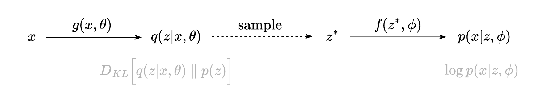
This is the variational autoencoder. It is variational because it computes a Gaussian approximation to the posterior distribution, and an autoencoder because it maps a data point $x$ into a lower-dimensional latent vector $z$, and then reconstruct $x$ from $z$. By maximizing the ELBO, we aim to improve the reconstruction quality while ensuring the approximation $q(z \vert x)$ closely matches the prior $p(z)$.
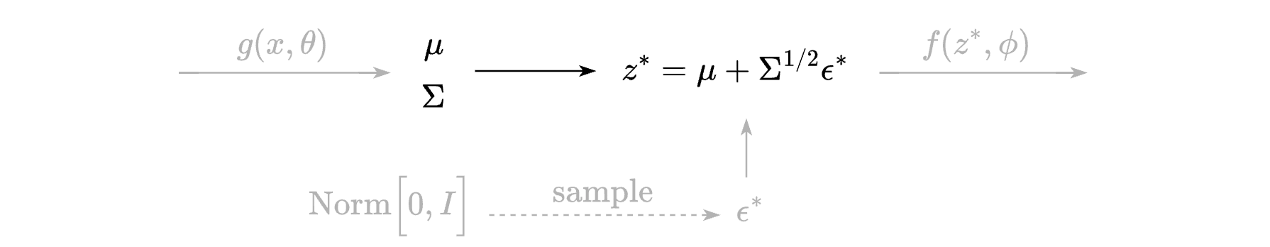
There is another challenge. The network involves a sampling step, making it non-differentiable. To address this, we use the reparameterization trick, which bypasses the sampling into another branch:
The reparameterization trick doesn’t work when the latent variable distribution is discrete. In such cases, we can use the log-derivative trick used from the REINFORCE algorithm, essential in policy gradient methods:
\[\gray \frac{\partial}{\partial \phi} E_{p(x\vert \phi)} \Big[ f(x) \Big] = E_{p(x\vert \phi)} \left[ f(x) \frac{\partial}{\partial \phi} \log p(x\vert \phi) \right]\]Details are in the appendix. Let $h(x, z) = \log p(x \vert z, \phi) + \log p(z) - \log q(z \vert x, \theta)$, then:
\[\gray \begin{align*} \frac{\part L}{\part \theta} &= \frac \part {\part \theta} E_{q(z\vert x, \theta)} \Big[ h(x, z) \Big] \\ &= E_{q(z\vert x, \theta)} \Big[ h(x, z) \frac \part {\part\theta} \log q(z \vert x, \theta)\Big] \\ &\approx \frac 1 N \sum_i h(x, z_i) \frac \part {\part\theta} \log q(z_i \vert x, \theta) \end{align*}\]This affects only the gradient calculation of the encoder parameters. We use the encoder once to calculate $\mu$ and $\Sigma$ of $q(z \vert x)$ then we sample $N$ observations $z_i^\star$ from $q(z\vert x)$. For each $z_i^\star$, we call the decoder to calculate $h(x, z_i^\star)$. However, REINFORCE tends to have higher variance, leading to more unstable training. To mitigate this, we may need more samples for reliable gradient estimates.
Applications
One application of VAEs is sample probability estimation. Unlike normalizing flows, there is no direct way to derive the probability, but it can be estimated effectively.
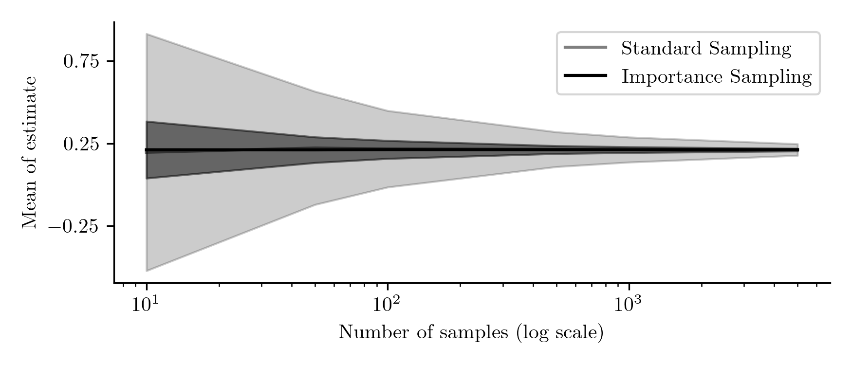
Theoretically, we could estimate $p(x)$ directly by sampling from the prior $p(z)$, but this is highly inefficient. Due to the curse of dimensionality, we would likely draw a point $z$ for which $p(x\vert z)$ is negligible, contributing little to the integral, leading to unstable estimates. Instead, we use importance sampling with a distribution that focuses on regions where $p(x\vert z)$ is high. A good choice is the variational posterior $q(z\vert x)$, computed by the encoder:
\[p(x) = \int p(x\vert z)p(z) dz = \int q(z\vert x)\frac{p(x\vert z)p(z)}{q(z\vert x)}dz = \mathbb{E}_{q(z\vert x)} \left[ \frac{p(x\vert z) p(z)}{q(z\vert x)} \right] \approx \frac{1}{N} \sum_{n=1}^{N} \frac{p(x\vert z_n) p(z_n)}{q(z_n \vert x)}\]Sample probability estimation can be used for evaluating model quality through estimating the log-likelihood of test data or for anomaly detection. See an example of importance sampling in the appendix.
The VAE can generate new examples. We sample $z^\star$ directly from the prior $p(z) = \text{Norm}_z \big[0, I\big]$ and pass it through the decoder to compute the mean $\mu = f(z^\star, \phi)$, then sample from $p(x\vert z, \phi) = \text{Norm}_x \big[\mu, \sigma I\big]$.
For image data, the generated samples are often of low quality, mainly because both the prior and the posterior are Normal distributions. The prior does not precisely describe the latent variable distribution the decoder expects - it should be the complex mixture of Gaussians rather than the prior $p(z)$ used as the reference during training. Moreover, the decoder returns a mean representing a blurred image, and sampling from the posterior adds Gaussian noise, further degrading visual quality.
VAEs provide better outcomes when using the aggregated posterior $q(z\vert \theta) = \frac 1 N\sum_i q(z\vert x_i, \theta)$ instead of the prior. Although, significant improvements come from hierarchical priors, linking to diffusion models we’ll explain in a following post.
Resynthesis is another powerful application of VAEs. After encoding a sample $x$ into latent variables $z$, we can manipulate these variables to generate a new example with specific features. The latent space is low-dimensional and largely disentangled, making it easier to isolate and modify particular attributes. For example, by averaging the latent variables of examples sharing a target feature (like a smile in portraits), we can derive a latent vector representing that feature. Adding this vector to the latent representation of an original image allows us to embed the desired feature into the generated output.
For audio data, VAEs are useful in voice cloning, where they encode speech into a latent space that captures speaker-specific features like timbre and pitch. Once encoded, we can manipulate the latent variables and resynthesize speech in the target voice.
Appendix
Jensen’s inequality. If $g$ is a concave function, then:
\[g(EX) \ge E [g(X)]\]Proof. Since $g$ is concave, all tangent lines to $g$ lie above the curve. Consider the tangent line at $(E[X],\ g(E[X]))$, defined as $f(x) = a + bx$. Because $f(x)$ lies above $g(x)$, we have $g(X) \le f(X)$ for all $X$. Taking expectations,
\[E[g(X)] \le E[a + bX] = a + bEX = g(EX)\]Now, let $Y= g(X) - f(X)$ so $Y \ge 0$. If $E(Y)=0$, then $P(Y =0)=1$, meaning equality holds if and only if $P(g(X) = f(X)) = 1$. $\blacksquare$
The figure on the left illustrates the concave function $g(X) = \log X$, with a tangent line at $ (EX, \ g(EX))$. As shown, the tangent line is always above the log curve for all values of $X$, meaning that the random variable $g(X)$ is upper-bounded by the random variable $f(X)$. Since $f$ is linear, the linearity of expectation gives us $E\big[ f(x)\big] = f(EX)$. Because $f$ is tangent to $g$ at $EX$, we have $f(EX) = g(EX)$.
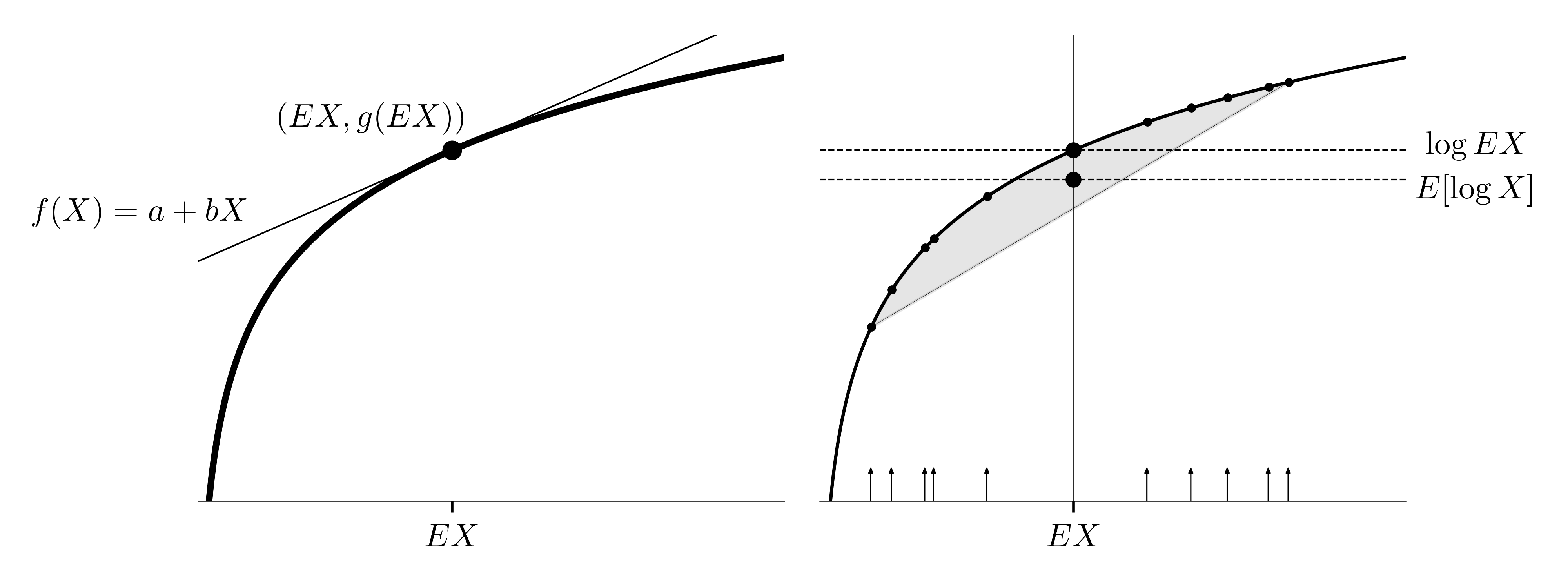
In other words, as shown in the figure on the right, any straight line connecting two points on the curve lies below the curve. The gray region under the curve represents the inequality: when taking a few observations of $X$ and applying the logarithmic transformation, the convex combination (weighted average) of the transformed values will fall below the curve, illustrating that $E[\log X] \le \log(EX)$. Think of the weighted average as a combination of averages between pairs of points:
\[\gray a_1(a_2 x_1 + (1-a_2)x_2) + a_3(a_4x_3 + (1-a_4) x_3) + \ldots\]For each pair, we draw a line and put a point at $a_{2n}$, with size $a_{2n+1}$. Since all points lie within the gray region, their average must also be within the region.
The KL divergence. If $p(x) = \text{Norm}_x \big[0, I \big]$ and $q(x) = \text{Norm}_x \big[\mu, \Sigma \big]$, we have:
\[D_{KL}\Big[ q(x) \| p(x)\Big] = \frac 1 2\Big( \text{Tr}(\Sigma) + \mu^T\mu - D_x - \log\vert \Sigma\vert \Big)\]Proof. The multivariable normal distribution is given by:
\[\gray \text{Norm}_{ x}\Big[\mu, \Sigma \Big] = \frac{1}{(2\pi)^{D/2}\vert \Sigma\vert ^{1/2}} \exp \Big[- \frac 1 2 ( x - \mu)^T\Sigma^{-1}( x - \mu)\Big]\]The exponential term returns a scalar that decreases as $ x$ moves away from the mean $\mu$, while the normalizing coefficient ensures the function sums to one. Using this definition for $\log p(x)$ and $\log q(x)$, the KL divergence between $q$ and $p$ becomes:
\[E_{q( x)}\Big[ \log \frac{q( x)}{p( x)}\Big] = \frac 1 2\Big( E\Big[ x^T x\Big] - E\Big[( x - \mu)^T\Sigma( x - \mu)\Big] + \log \vert \Sigma\vert \Big)\]For the first expectation, adding and subtracting $ \mu^T\mu$, we have:
\[\gray E\Big[ x^T x\Big] = \mu^T\mu \gray+ \underbrace{E\Big[( x - \mu)^T( x - \mu)\Big]}_{\black \sum_i E(x_i - \mu_i)^2 = \sum_i \Sigma_{ij} = \text{Tr}(\Sigma)}\]Decomposing the second expectation into the sum of individual terms,
\[\gray E\Big[ ( x-\mu)^T\Sigma^{-1}( x-\mu)\Big] = E\left[\sum_{i, j} (x_i - \mu_i)\Sigma^{-1}_{i,j}(x_j - \mu_j) \right] = \sum_{i,j} \Sigma^{-1}_{i, j} \Sigma_{i, j}\]Since $\sum_{i, j}A_{i, j}B_{i, j} = \text{Tr}(A^TB)$, and $\Sigma$ is symmetric,:
\[\gray \sum_{i,j} \Sigma^{-1}_{i, j} \Sigma_{i, j} = \text{Tr}(\Sigma^{-T}\Sigma) = \text{Tr}(I) = D_x\]Substituting these results into the KL divergence expression, we reach the final form. $\blacksquare$
The REINFORCE algorithm.
\[\frac{\partial}{\partial \phi} E_{p(x\vert \phi)} \Big[ f(x) \Big] = E_{p(x\vert \phi)} \left[ f(x) \frac{\partial}{\partial \phi} \log p(x\vert \phi) \right]\]Proof. The expectation of $f(x)$ with respect to $p(x \vert \phi)$ is defined as:
\[\gray E_{p(x\vert \phi)} \Big[ f(x) \Big] = \int f(x)p(x \vert \phi)dx\]We now differentiate both sides with respect to $\phi$, applying the product rule of differentiation:
\[\gray \frac \part {\part \phi} E_{p(x\vert \phi)} \Big[ f(x) \Big] = \int f(x)\frac \part {\part \phi}p(x \vert \phi)dx\]The key step is recognizing that:
\[\gray \frac \part {\part\phi} \log p(x \vert \phi) = \frac 1 {p(x \vert \phi)} \frac{\part}{\part \phi} p(x\vert \phi)\]Substituting this into the integral, we get:
\[\gray \frac \part {\part \phi} E_{p(x\vert \phi)} \Big[ f(x) \Big] = \int f(x) p(x \vert \phi)\frac \part {\part \phi} \log p(x \vert \phi)dx\]Recognizing this as the expectation with respect to $p(x \vert \phi)$, we obtain the final form. $\blacksquare$
Importance sampling. Suppose we need to estimate $E_{p(x)}\big[f(x)\big]$, where $p(x) = \text{Norm}_x[0,1]$ and the function $f(x) = 10 \cdot \exp\left(- (x - 3)^4\right)$ is unknown. However, we know that the distribution $q(x) = \text{Norm}_x[3,1]$ likely covers regions where the function takes larger values. By leveraging this information, we can improve the accuracy of our estimate:
\[E_{p(x)}\big[f(x)\big] = E_{q(x)}\Big[f(x) \frac {p(x)}{q(x)} \Big]\]Importance sampling is most effective when the auxiliary distribution $q(x)$ closely matches the high-value regions of the target function $f(x)$. This allows us to concentrate sampling efforts where the function is most significant, reducing variance and making the estimation more efficient compared to directly sampling from $p(x)$.