Optimization methods
Neural network loss functions are non-convex and complex, leaving no choice but to use numerical methods to find a solution. We often use iterative gradient-based methods, which involve two main steps: (i) calculating the gradients and (ii) updating the parameters. Given the gradient of all network parameters at time $t$, the vanilla Gradient descent algorithm is as follows:
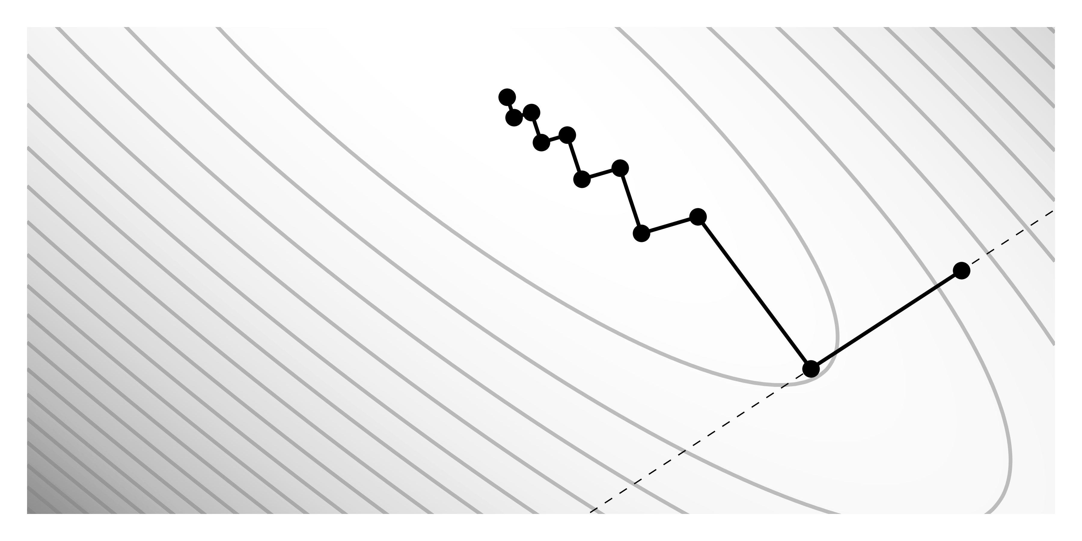
\[\v \phi_{t+1} \gets \v \phi_t - \alpha \nabla L[\v \phi_t]\]The learning rate $\alpha$ can be a constant hyperparameter, or we can use, for example, a line search. It does a few additional model calls to find the minimum of the loss function along the gradient direction. The figure shows the simple convex loss surface, where the dashed lined represents the gradient direction for the first point. The second point reaches the minimum along this line, defining $\alpha$. However, for non-convex and high-dimensional spaces, line search is either impractical or ineffective.
Iterative gradient-based methods inherently suffer from relying solely on the gradient as the sole source of information. The optimization process can get stuck in local minima or flat regions when the gradient fails to provide useful information for improvement. Additionally, the gradient describes a loss function at a specific point, indicating the correct direction of progress for infinitesimal parameter changes whereas optimization algorithms use a finite step size:
\[\nabla L[\v\phi] \black d\v\phi\ \approx\ \nabla L[\v\phi] \black\Delta\v\phi\]Too-small learning rates prolong the training process, and for non-convex functions, they increase the likelihood of getting stuck in local minima. Too-large learning rates causes “bouncing”, which can block learning entirely. Variations of optimization algorithms are designed to address these issues.
Stochastic gradient descent
Stochastic gradient descent (SGD) adds noise to the gradient. At each step, we approximate the gradient using a subset of the training data, drawing without replacement to form a mini-batch. Since observations are independent, individual losses can be summed up, resulting in:
\[\v \phi_{t+1} \gets \v \phi_t - \alpha \sum_{i \in B} \frac{l_i[\v \phi_t]}{\part \v \phi}\]SGD has several pleasing features. It improves the fit to subsets of the data, is less computationally expensive, can (in principle) escape local minima, and reduces chances of getting stuck near saddle points. As the observations in a batch change, so does the loss function. By drawing a mini-batch, we indirectly draw which loss function we minimize at each step. To get stuck, all of possible loss functions would need to be flat.
Momentum
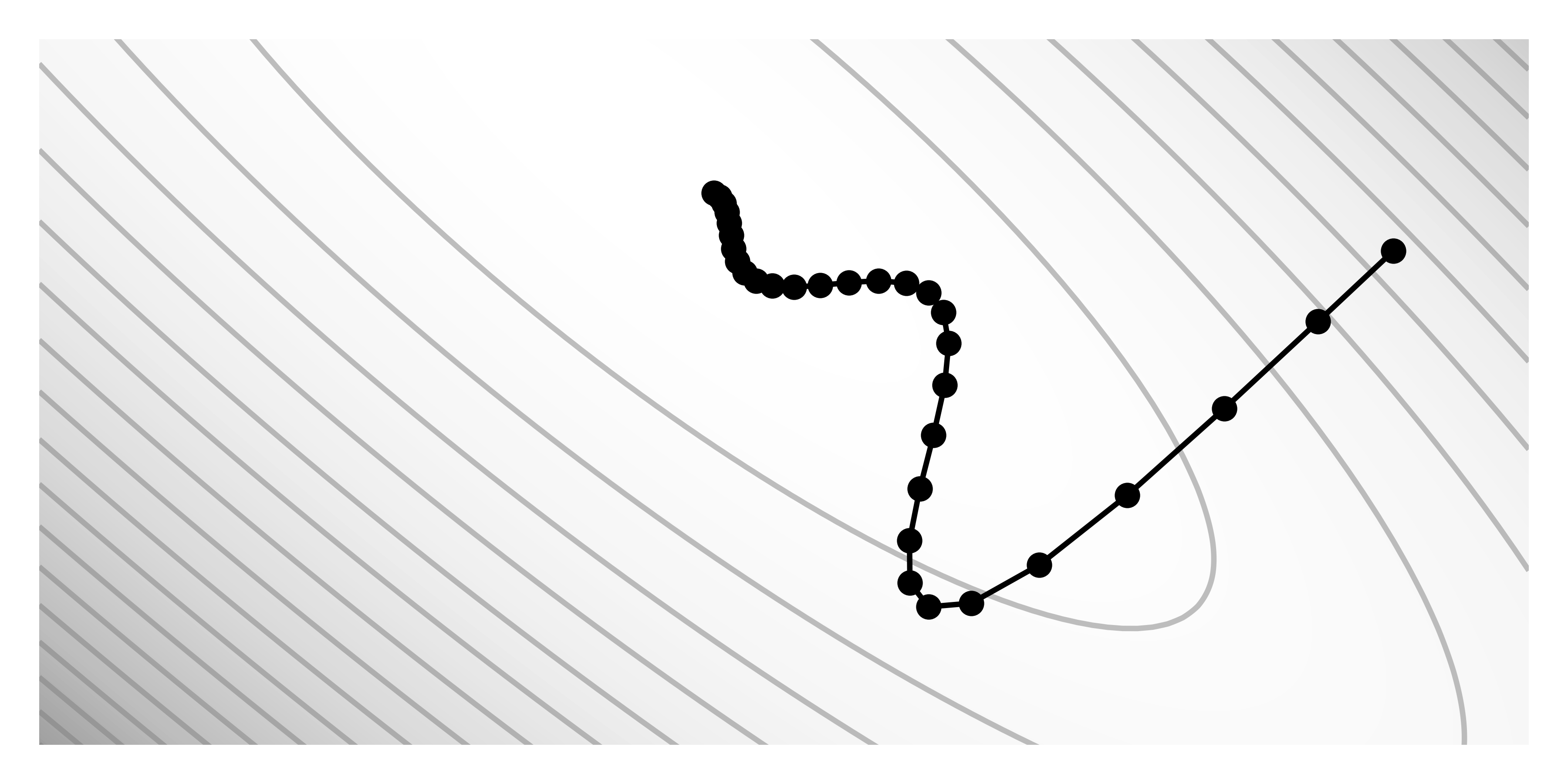
SGD suffers from oscillations due to sharp direction changes since each update is independent. A momentum term smooths the trajectory. The gradient step becomes an infinite weighted sum of all previous gradients, where the weights get smaller as we move back in time:
\[\v m_{t+1} \gets \beta \v m_t + (1-\beta) \nabla L[\v \phi_t] \\[5px] \v \phi_{t+1} \gets \v \phi_t - \alpha \v m_{t+1}\]The parameter $\beta \in [0, 1)$ controls the degree to which the gradient is smoothed over time. With $\beta=0.9$, the influence of a gradient $50$ steps ago is below $1\%$. Momentum accumulates gradients that go into a similar direction, diminishing those that contradict each other.
Nesterov momentum introduces a clever tweak. It computes the gradient $\nabla L[\cdot]$ at the position $\v \phi_t - \alpha \beta \v m_t$, rather than at $\v \phi_t$. Using the analogy of steering a car, we correct our direction based on where we’ll be shortly, not where we are now. This method refines trajectory correction, making the optimization process more efficient.
Adaptive moments
A constant step size across all dimensions may not be ideal, as a loss function may exhibit varying sensitivity across different dimensions. Sensitive dimensions might experience “bouncing” with a too-large learning rate, hampering learning, while less sensitive dimensions could require an impractically long time to converge if the learning rate is too low. Adaptive moment estimation (Adam) addresses this issue by adjusting the step size according to gradient magnitudes, using the second moment estimate; the variance measure for each parameter:
\[\v v_{t+1} \gets \gamma \v v_t + (1-\gamma) \big(\nabla L[\v \phi_t]\big)^2\]Combining the first and second moment estimates, the parameter update is:
\[\v \phi_{t+1} \gets \v \phi_t - \frac{\alpha}{\sqrt{\v {\tilde{v}_{t+1}}} + \epsilon}\v {\tilde{m}}_{t+1}\]Both estimates are initialized with zeros, resulting in biased and smaller estimates early in training. Adam corrects this bias by adjusting each estimate, which has a diminishing effect over time:
\[\tilde {\v m}_{t+1} \gets \frac{\v m_{t+1}}{1 - \beta^{t+1}} \\ \tilde {\v v}_{t+1} \gets \frac{\v v_{t+1}}{1 - \gamma^{t+1}} \\\]Additionally, implementing a learning rate warm-up strategy can further mitigate the impact of initial bias, gradually increasing the learning rate at the start of training to improve stability and performance. For details on using L2 regularization, see AdamW.
Appendix
A function is convex if no chord, line segment between two points on the surface, intersects a function. Let $\v \phi_1$ and $\v \phi_2$ be two possible sets of parameters where $\v \phi_t = t \v \phi_1 + (1-t)\v \phi_2$. The function is convex if for all $\v \phi_1$ and $\v \phi_2$, and for any $0 \le t \le 1$, the condition $L(\v \phi_t) \le tL(\v \phi_1) + (1-t)L(\v \phi_2)$ holds. Alternatively, we may verify convexity by checking if the Hessian $\v H[\v \phi]$ is positive definite for all possible parameters.