Loss functions
In supervised learning, the goal is to find the conditional distribution $p(\v y \mid \v x)$. The distribution may take various complex forms. We therefore approximate it by the distributions we know, e.g. the Normal distribution. Among different parameterizations $\theta$, we search for the one $q_\theta(\v y \mid \v x)$ that is closest to the true distribution.
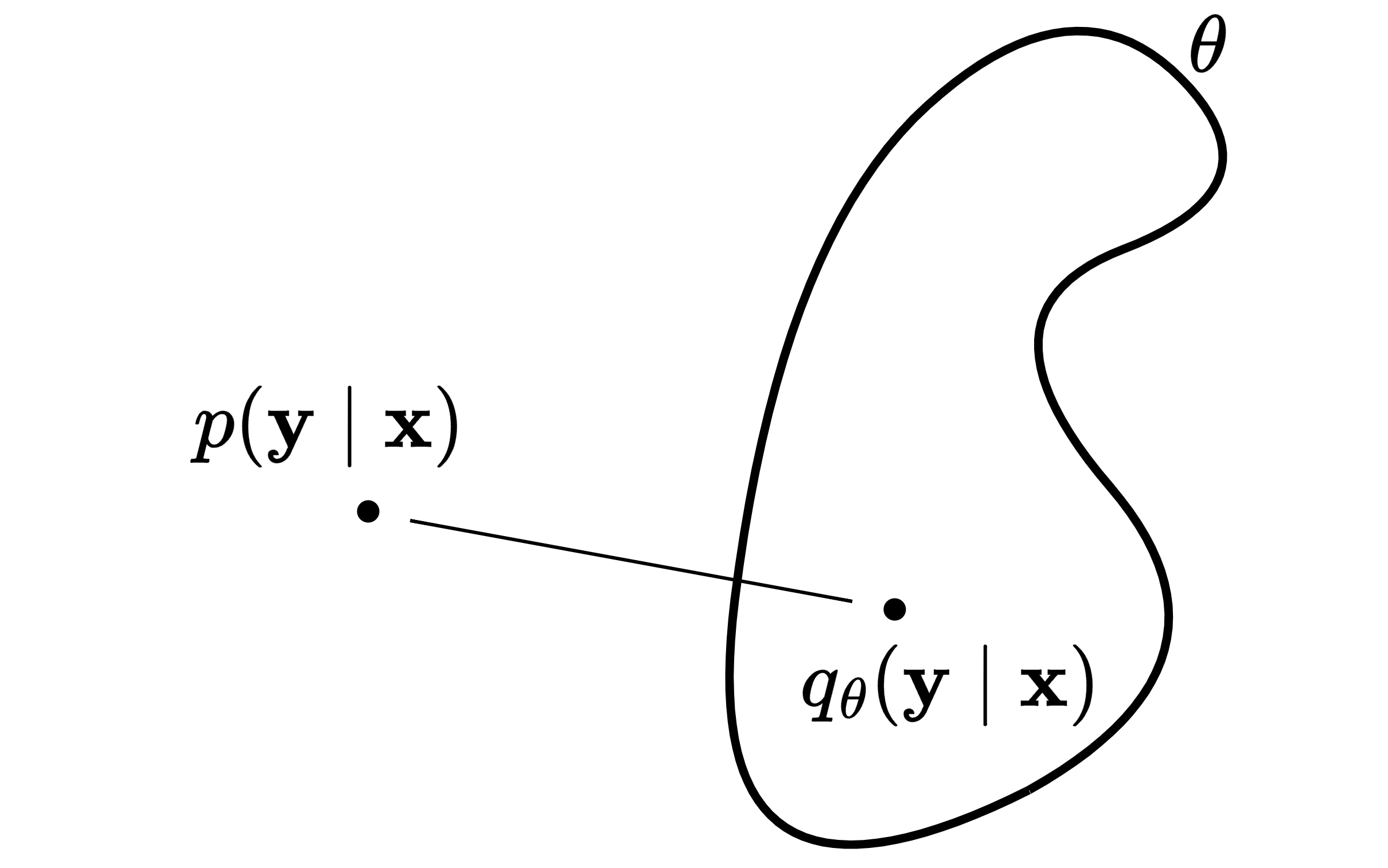
A model given $\v x$ predicts parameters $\theta$ to define the conditional distribution $q_{\theta}(\v y \mid \v x)$. The model is a transformation, the one-to-one mapping $\theta = f[\v x, \v \phi]$ with parameters $\phi$. This means $\theta$ is also a random variable, like $\v x$. Therefore, our goal is to find the model parameters $\phi$ that for each observation $\v x_i$ give the best $\theta_i$.
Maximum likelihood
To train the model, we need the loss function $L[\v \phi]$ that measures how well a model predicts parameters $\theta_i$. However, the problem is that these parameters $\theta_i$ are unknown.
\[\v x_i \rightarrow \hat\theta_i \quad \theta_i \rightarrow \v y_i\]One approach is to use the maximum likelihood estimation (MLE) and assume that these parameters must maximize the likelihood of observing the training data $\lbrace \v x_i, \v y_i \rbrace$. In practice, we often assume that observations are i.i.d., so the probability of observing the training data can be split into independent components:
\[p(\v y_1, \ldots \vert \v x_1, \ldots)= \prod_i p(\v y_i \vert \v x_i)\]According to MLE, the best model parameters $\phi$ produce for each $\v x_i$ distribution parameters $\theta_i$ that make $\v y_i$ the most likely. In other words, the distribution $q_{\theta_i}(\v y \mid \v x_i)$ has the maximum value at $\v y_i$. Using $\text{argmax}$,
\[\begin{align*} \argmax{\phi}\bigg[ \prod_i q(\v y_i \vert \v x_i, \phi) \bigg] \end{align*}\]Maximizing the likelihood and log-likelihood is equivalent since the log function is monotonically increasing. Because we work with a loss function (which we minimize), we multiply by $-1$ to change $\text{argmax}$ into $\text{argmin}$.
\[\argmax{\phi}\bigg[ \prod_i q(\v y_i \mid \v x_i, \v \phi) \bigg] = \argmin{\phi}\bigg[ -\sum_i \log q(\v y_i \mid \v x_i, \v \phi) \bigg]\]This gives us the numerically stable negative log-likelihood loss (NLL) function:
\[L[\phi] = -\sum_i \log q(\v y_i \mid f[\v x_i; \v \phi])\]To sum up, the MLE assumes that the observed data points must be the most likely - a premise that likely might not be true. Less probable distribution parameters, while less likely given a specific dataset $\lbrace \v x_i, \v y_i \rbrace$, may generalize better across other datasets. See the Bayesian linear regression post for an alternative approach.
\[\begin{align*} \gray\underbrace{\black\space \v x_i \rightarrow \hat\theta_i \overset{\text{MLE}}{\approx} \v\theta_i \ }_{\text{training}} \black\to \v y_i\space \end{align*}\]After the training, we find the most likely model parameters $\v\phi$. During inference, the model uses them to estimate the distribution parameters $\theta$. We may return either the full distribution or its most likely value:
\[\hat {\v y} = \argmax y\Big[ q_{\theta}(\v y \mid \v x) \Big]\]Example
The conditional distributions can take various forms. We often assume they belong to the same distribution family as the marginal distribution of $\v y$. Let $y$ be a random variable that marginally follows the Beta distribution. In that case, a model estimates two parameters $a_i$ and $b_i$ of the conditional Beta distribution given $\v x_i$. For the training, we can derive the negative log-likelihood loss function involving the Beta distribution $q(y) \propto y^{a-1}(1-y)^{b-1}$:
\[L[\v\phi] = -\sum_i \log q(\v y_i \mid \v\theta) = -\sum_i \bigg[ (a-1)\log y_i + (b-1)\log(1-y_i)\bigg]\]The figure shows the predicted Beta conditional distribution given $\v x_i$. The predicted parameters $a_i$ and $b_i$ are inaccurate because the likelihood of $y_i$ is low, resulting in a high loss. These parameters would be perfect if $y_i$ were $0.2$ but not $0.7$. In other words, the parameters of the conditional distribution that we assume to be true are those for which $y_i$ is most likely. For example, the parameters $a_i=2$ and $b_i=5$ would minimize the loss, as well as other configurations that satisfy $(a-1)/(a+b-2) = 0.7$. The MLE assumption allows for a set of valid parameter configurations rather than a single specific one.

During inference, we may either return the most likely value or the full distribution to quantify uncertainty. When returning the maximum of a distribution, some distributions offer a closed form. For the Beta distribution, the most likely value (mode) is given by $(a-1)/(a+b-2)$.
Regression
The negative log-likelihood loss functions can be derived for various distributions. For regression, we may assume a Normal distribution with constant variance, so the model estimates only the mean. Ignoring all constants and using $q(y) \propto \exp[-(y - f[\v x, \v \phi])^2]$, we aim to minimize:
\[L[\v\phi] = -\sum_i \log q(\v y_i \mid \v\theta)= \sum_i (y_i-f[\v x_i; \v\phi])^2\]The NLL loss function with a Normal conditional distribution aligns with the least squares method, creating a bridge between probabilistic approaches and traditional regression analysis. When a model predicts both the mean and the variance (e.g. a heterogeneous Normal distribution), the variance serves as a measure of uncertainty, providing insights into the model’s confidence.
Classification
In binary classification, we may use the Bernoulli distribution $p(y) = \lambda^y(1-\lambda)^{1-y}$. Its parameter $\lambda$ must stay between $0$ and $1$. To achieve this, we add the sigmoid activation at the end of the network, such as the logistic function $\sigma(x) = 1/(1 + e^{-x})$. For $\lambda_i = \sigma(f[\v x_i; \v\phi])$, the loss function becomes:
\[\begin{align*} L[\v \phi] = -\sum_i\bigg[ y_i \log\lambda_i + (1-y_i) \log(1-\lambda_i) \bigg] \end{align*}\]For multiclass classification, we use the Categorical distribution with the softmax activation function instead. The NLL loss function encourages the model to increase the logit of the correct class relative to others.
\[L[\phi] = -\sum_i \bigg[ f_{y_i}[x_i;\phi] -\log\left(\sum_d \exp(f_d[x_i; \phi])\right)\bigg]\]Difference between distributions
Instead of maximizing the likelihood of observing data, we can alternatively minimize the distance between the true and estimated distributions, $p$ and $q$. The true empirical distribution is represented as a set of Dirac delta functions, forming infinite peaks at the positions of observations $y_i$:
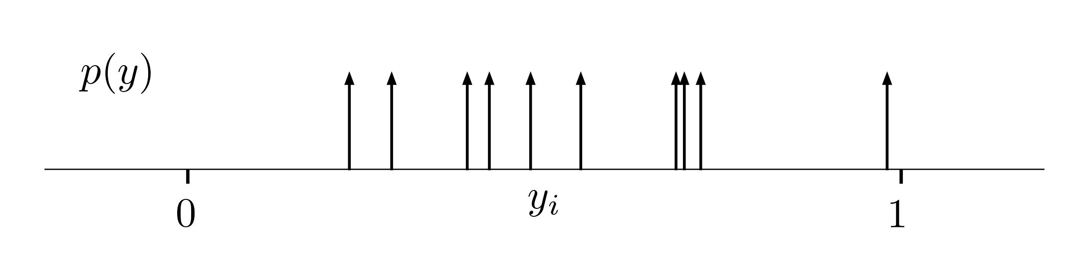
We can measure the difference between distributions using the KL-divergence. As before, the model predicts the parameters $\v \theta = f[\v x_i; \phi]$ that we use in the predicted conditional distribution $q$ of $\v y_i$ given $\v x_i$. Removing constants, and picking “values” of a continuous function through a set of Dirac delta functions, we obtain:
\[\begin{align*} \hat \phi &= \argmin \phi \left[\int p(y)\log \frac{p(y)}{q(y|\v \theta)} dy \right] \\ &\gray = \argmin \phi \left[- \int p(y)\log [{q(y|\v \theta)}] dy \right] \quad\quad\text{cross-entropy} \\ &\gray = \argmin \phi \left[- \int \left(\frac 1 n \sum_{i=1}^n \delta[y - y_i] \right)\log[{q(y|\v \theta)}] dy \right]\\ &= \argmin \phi \left[- \sum_{i=1}^n \log[q(y_i|\v \theta)] \right] \end{align*}\]This shows that minimizing the KL-divergence between the true and estimated distributions is equivalent to minimizing the Negative Log-Likelihood loss function (see the log-sum-exp trick).
Appendix
The Kullback-Leibler divergence measures a distance between two probability distributions $p(x)$ and $q(x)$. Both functions are defined over the space $x$ but represent different random variables. They share a common support, allowing for comparison. \(D_{KL}\bigg[p(x)\ \|\ q(x) \bigg] = \int p(x) \log \frac{p(x)}{q(x)} dx\)
The probability distance must be greater than or equal to zero. This can be shown using $-\log z > 1-z$,
\[\gray \int p(x)\bigg(-\log\frac{q(x)}{p(x)}\bigg) dx \ge \int p(x) \bigg(1- \frac{q(x)}{p(x)}\bigg) dx = 0\]The KL-divergence is not symmetric. To illustrate this, consider $p(x)$ and $q(x)$ as the true and predicted normal distributions, with $p(x)$ having two modes and $q(x)$ having one mode.
Using the forward divergence $D_{KL}(p\ |\ q)$ as the loss function, the trained $q(x)$ would fit the mean of the two modes, maximizing recall. Consider a situation where $p(x) \gg q(x)$, for example, when $q(x)$ is close to zero and $p(x)$ is not. The match between them $q(x) / p(x)$ will approach zero, leading to the high cost $-\log(q(x)/p(x))$. As the model aims to avoid such situations, it assigns $q(x) > 0$ wherever $p(x) > 0$.
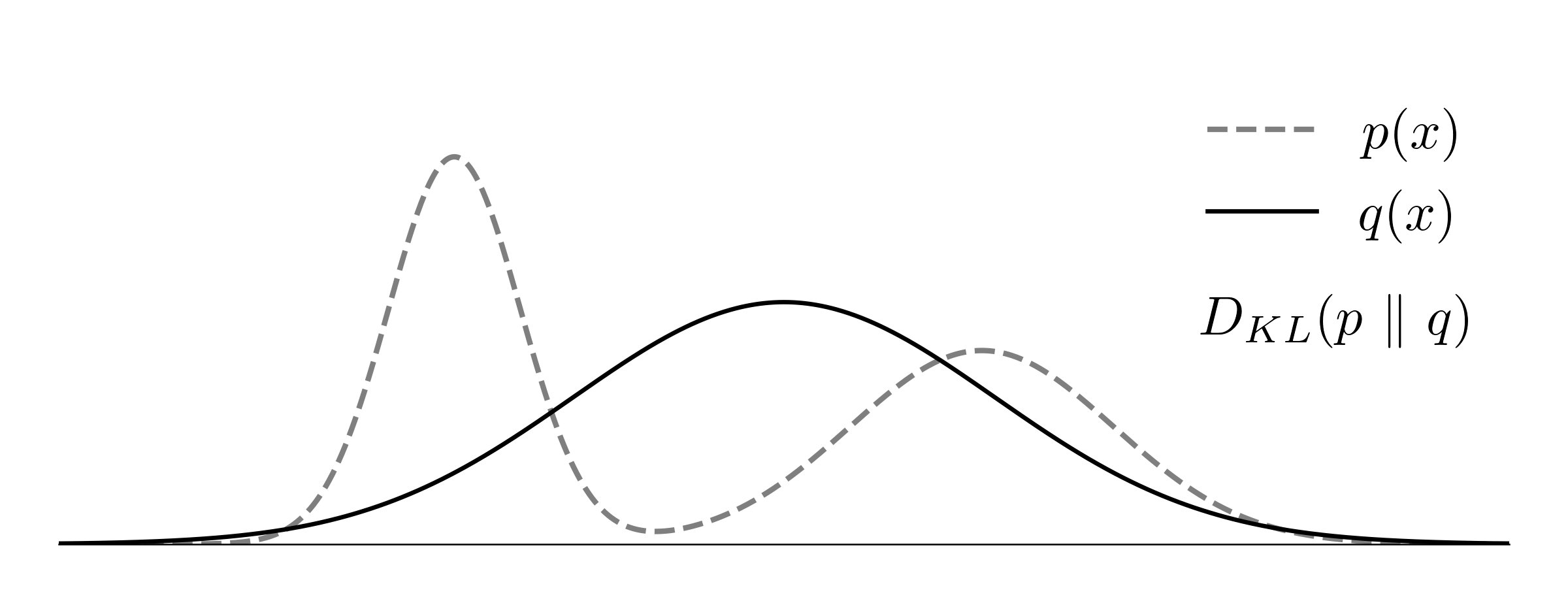
In the reversed divergence $D_{KL}(q\ |\ p)$, the model can select and focus on a subregion of the support of $p$, as the expectation is taken with respect to the random variable $q(x)$. As a result, the trained $q(x)$ would closely match one of the two modes, maximizing precision.
The log-sum-exp trick is a numerical stability technique used when computing the logarithm of a sum of exponentials - a common case in softmax and cross-entropy loss calculations. By subtracting $ m = \max_i x_i$ from each element $x_i$, we keep the exponentials within a manageable range, preventing numerical overflow and ensuring stable gradient computations during training:
\[\log \sum_i e^{x_i} = m + \log \sum_i e^{x_i - m}\]For a single sample $\v x$, the cross-entropy loss becomes:
\[\ell(\v x) = - \log q(\v x) = -\log \frac {e^{x_i}}{\textstyle\sum_j e^{x_j}} = - x_i + m + \log \textstyle\sum_j e^{x_j-m}\]where $x_i$ is the logit for the correct class. In PyTorch, we can achieve this in two ways. First, by applying $\text{LogSoftmax}$ (with incorporates the log-sum-exp trick) followed by $\text{NLLoss}$,
log_softmax = nn.LogSoftmax(dim=-1)
loss_fn = nn.NLLLoss()
loss = loss_fn(log_softmax(logits), target)
where $\text{NLLoss}$ is simply $f(\v x) = - x_i$ when the correct class is $i$. Alternatively, we can directly feed raw logits into $\text{CrossEntropy}$, which internally applies the softmax and computes the loss:
loss_fn = nn.CrossEntropy()
loss = loss_fn(logits)