Diffusion models

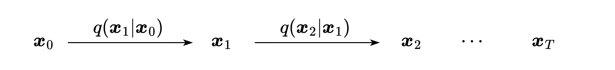
Denoising diffusion probabilistic models, like other generative models, aim to learn a data distribution $q(\v x_0)$. The key idea is to generate a sequence of latent variables $\v x_t$ starting from $\v x_0$, where the relationships between them are predefined. These variables form a Markov chain, with the transition between them defined as:

\[\begin{align*} \v x_t \coloneqq \sqrt{1 - \beta_t}\ \v x_{t-1} + \sqrt {\beta_t}\ \v\epsilon && \text{where} && \v\epsilon \sim \Norm 0 I \end{align*}\]

With each step $t$, we add noise to the original example $\v x_0$, and the amount of noise is controlled by the coefficient $\beta_t \in [0, 1]$. This is the forward process, which gives us the chain of latent variables:

The aim is to find a distribution $p(\v x_{0\ldots T})$ over data and latent variables that closely matches the true distribution $q(\v x_{0\ldots T})$ because then a data distribution $p(\v x_0)$ can be derived from marginalizing over latent variables $\v x_{1\ldots T}$. In other words, once we learn the distribution over latent variables, we can use them to predict the likelihood of $\v x_0$. The log likelihood is estimated by calculating the expectation over the conditional log likelihoods given $\v x_1$. How well we model the distribution over latent variables determines how tight this bound is.

\[\begin{align*} \log p(\v x_0^{(i)}) &\ge E_{q(\v x_1 | \v x_0^{(i)})}\Big[\log p(\v x_0^{(i)}|\v x_1) \Big] \gray - \text{mismatch} \end{align*}\]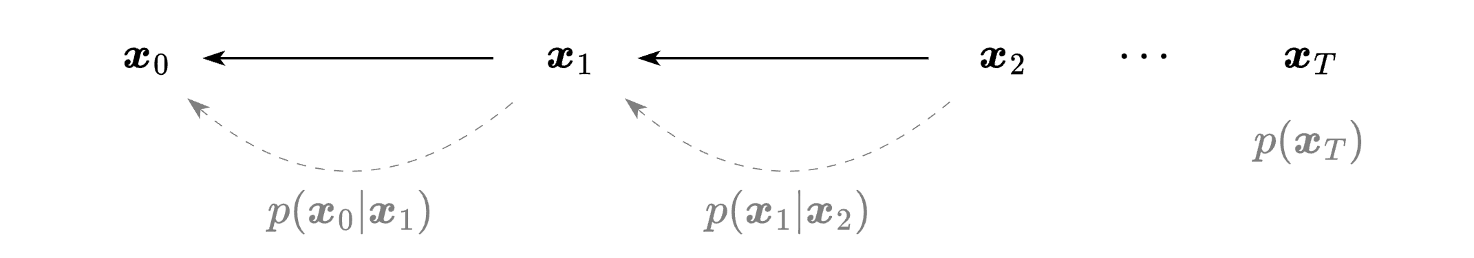

This is the idea also used in VAEs but here we marginalize many latent variables, not just one, and the encoder becomes a predefined Markov process. In VAEs, the decoder has one hard problem - learning the mapping $\v x_T \to \v x_0$. In diffusion models, the decoding is divided into $T$ simper sub-problems $\v x_t \to \v x_{t-1}$.

Converging to Normal

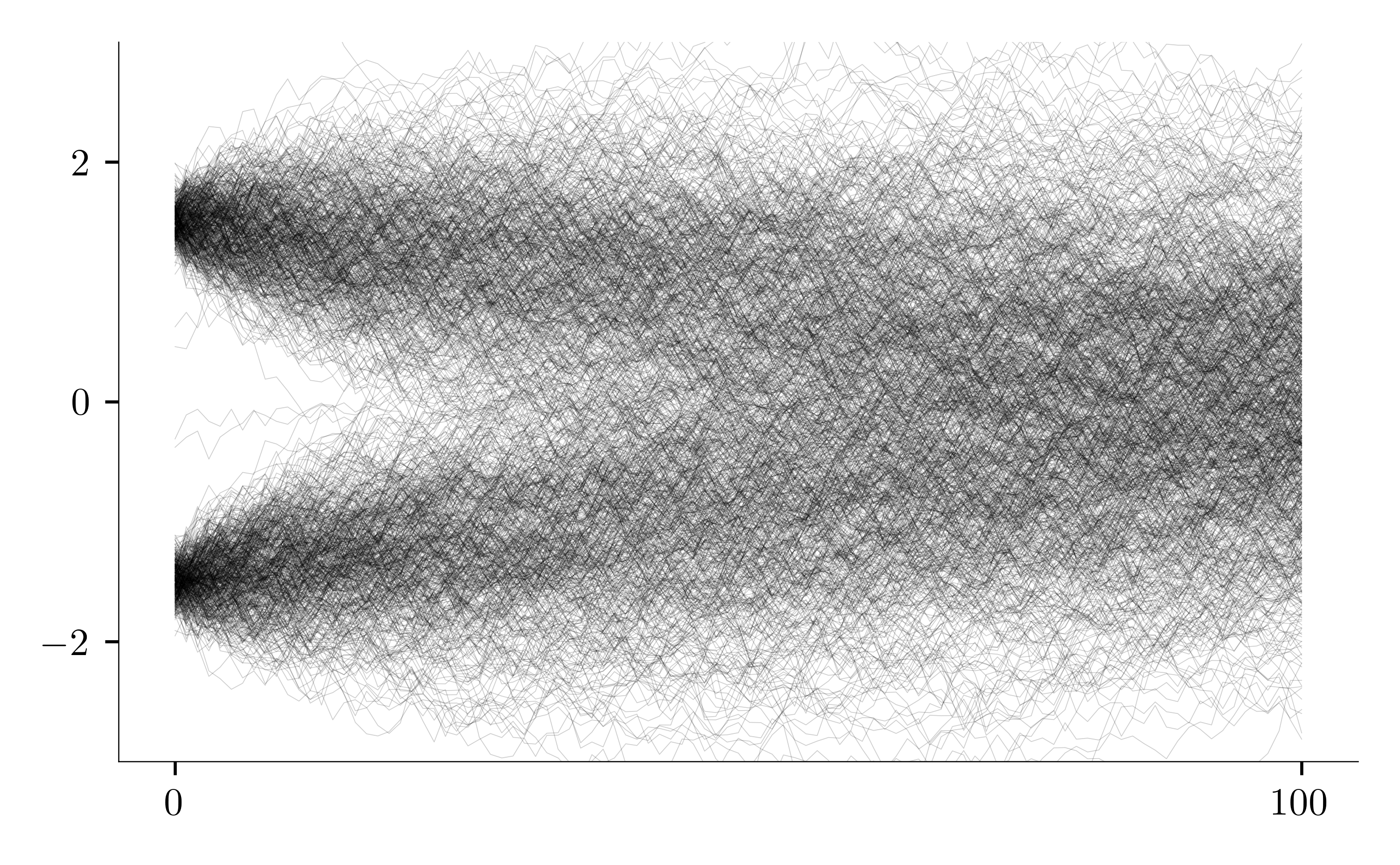
The diffusion process is highly effective because it transforms a complex data distribution into a simpler one, step by step, iteratively adding noise until it eventually reaches a standard Normal distribution. To see this, let’s define the joint distribution of latent variables given $\v x_0$ using the relationships between the variables:

\[\begin{align*} q(\v x_{1\ldots T}|\v x_0) \coloneqq \prod_{t=1}^T q(\v x_t | \v x_{t-1}) &&\text{where}&& q(\v x_t | \v x_{t-1}) = \Norm{\sqrt{1 - \beta_t}\v x_{t-1}}{\beta_tI} \end{align*}\]

The conditional distribution $q(\v x_t \vert \v x_{t-1})$ is a Normal distribution because, as mentioned earlier, the transition from $\v x_{t-1}$ to $\v x_t$ is a linear combination of the condition $\v x_{t-1}$ and the noise $\v \epsilon$, which is normally distributed. By marginalizing this joint distribution (see the appendix), we find a special property of the forward process:

\[\begin{align*} q(\v x_t | \v x_0) = \int q(\v x_{1\ldots t}|\v x_0) d\v x_{1\ldots(t-1)} = \Norm{\sqrt {\alpha_t} \v x_0}{(1-\alpha_t)I} &&\text{where}&& \alpha_t = \prod_{i=1}^t (1-\beta_i) \end{align*}\]

We call $q(\v x_t \vert \v x_0)$ the diffusion kernel. This kernel has two useful properties. First, it allows us to skip intermediate latent variables and calculate a conditional distribution directly. Second, as the forward process progresses, the conditional distributions $q(\v x_t \vert \v x_0)$ lose track of the condition $\v x_0$. Eventually, as $T$ becomes large, $\alpha_T$ approaches zero, and the conditional distribution effectively becomes the marginal:

\[\begin{align*} q(\v x_T | \v x_0) = \Norm 0 I &&\text{thus} && q(\v x_T | \v x_0)= q(\v x_T) \end{align*}\]

This is crucial since the diffusion process converges to a tractable and simple Normal distribution, from which we can easily sample during inference. The figure below illustrates the diffusion process: starting from a one-dimensional mixture of two Normal distributions, the diffusion process gradually blurs the distribution, moving it toward a standard Normal distribution.

Deriving the lower bound

Diffusion models, as other generative models, aim to learn a data distribution $q(\v x_0)$ by maximizing the log-likelihood of data. As in VAEs, we derive the probability $p(\v x_0)$ by marginalizing over the latent variables:

\[\begin{align*} \hat\phi = \argmax{\phi}\Big[\sum_{i=1}^N \log p(\v x_0^{(i)} | \phi)\Big] &&\text{where}&& p(\v x_0) = \int p(\v x_{0\ldots T}) d\v x_{1\ldots T} \end{align*}\]

In addition to learning a data distribution, generative models should provide a way to efficiently generate new examples. To achieve this and to match the properties of the true distribution $q(\v x_{0\ldots T})$, we define the model distribution $p(\v x_{0\ldots T})$ as a Markov chain in reverse, starting from $\v x_T$ and processing back to $\v x_0$:

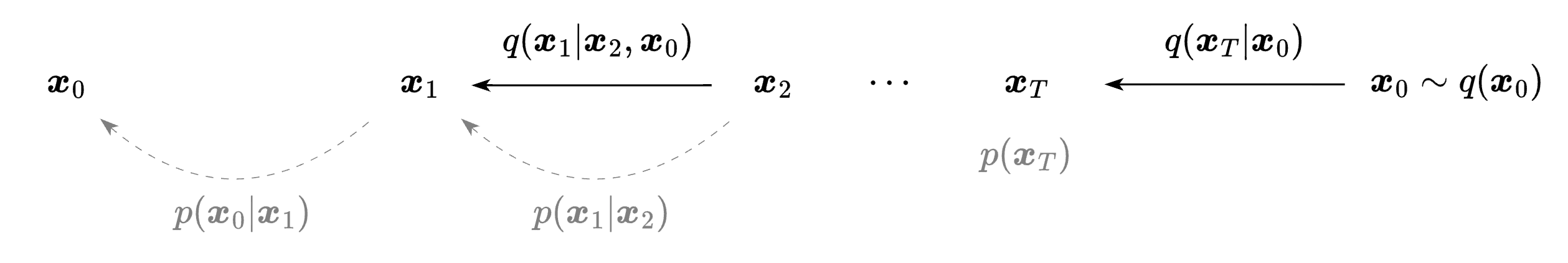
\[\begin{align*} p(\v x_{0\ldots T}) \coloneqq p(\v x_T)\prod_{i=1}^T p(\v x_{t-1}| \v x_t) &&\text{where}&& p(\v x_T) = \Norm 0 I \end{align*}\]

As shown earlier, the result of the forward process $q(\v x_T \vert \v x_0)$ is a standard Normal distribution, so it is reasonable to assume that the prior $p(\v x_T)$ is also a standard Normal distribution. This again highlights the importance of the diffusion process converging to a simple, tractable Normal distribution. With this assumption, we can assume a simple prior $p(\v x_T)$ from which we can easily sample and start the reverse process. Using ancestral sampling, we draw $\v x_T^\star \sim p(\v x_T)$, then sample $\v x_{T-1}^\star \sim p(\v x_{T-1}\vert \v x_T^\star)$, and so on until we generate $\v x_0^\star$ from $p(\v x_0 \vert \v x_1^\star)$.

Even though we can break the joint distribution into simpler components, we cannot maximize the log-likelihood directly because the integral is intractable. However, we can estimate the log likelihood using the Evidence Lower Bound (ELBO):

\[\begin{align*} \log p(\v x_0) &= \log\Bigg[ \int q(\v x_{1\ldots T} | \v x_0) \frac{p(\v x_{0\ldots T})}{q(\v x_{1\ldots T} | \v x_0)} d\v x_{1\ldots T}\Bigg] \\[3px] &\ge E_{q(\v x_{1\ldots T} | \v x_0)} \Bigg[ \log\frac{p(\v x_{0\ldots T} | \phi_{0\ldots T})}{q(\v x_{1\ldots T} | \v x_0)}\Bigg] = \text{ELBO}\big[\v \phi_{0\ldots T}\big] \end{align*}\]

The bound is tight if the conditional distributions given $\v x_0$ over latent variables $q(\v x_{1\ldots T} \vert \v x_0)$ and $p(\v x_{1\ldots T} \vert \v x_0)$ closely match. By rearranging the expectation, we obtain:

\[\gray \text{ELBO}\big[\v \phi_{0\ldots T}\big] = \log p(\v x_0) + E_{q(\v x_{1\ldots T} | \v x_0)} \Bigg[ \log\frac{p(\v x_{1\ldots T} | \v x_0)}{q(\v x_{1\ldots T} | \v x_0)}\Bigg]\]

Simplifying ELBO

We can simplify the ELBO by decomposing the distribution over latent variables given $\v x_0$:

\[q(\v x_{1\ldots T} | \v x_0) \coloneqq \prod_{t=1}^T q(\v x_t | \v x_{t-1}) = q(\v x_T | \v x_0) \prod_{t=2}^T q(\v x_{t-1} | \v x_t, \v x_0)\]

Here, we use a Markov chain property and Bayes’ rule to break down each term (for details, see the appendix). By substituting $p(\v x_{0\ldots T}) $ and $q(\v x_{1\ldots T} \vert \v x_0) $ into the ELBO, the log term simplifies to:

\[\gray \log\frac{p(\v x_{0\ldots T})}{q(\v x_{1\ldots T} | \v x_0)} = \log p(\v x_0 | \v x_1) + \Bigg(\sum_{t=2}^T \log \frac{p(\v x_{t-1}|\v x_t)}{q(\v x_{t-1}|\v x_t, \v x_0)}\Bigg) + \log\frac{p(\v x_T)}{q(\v x_T | \v x_0)}\]

For each term, the expectation is over all latent variables $q(\v x_{1\ldots T} \vert \v x_0) $. However, the variables that are not involved cancel out, leading us to:

\[\begin{align*} \text{ELBO}[\phi_{0\ldots T}] = E_{q(\v x_1|\v x_0)}\big[\log p(\v x_0|\v x_1) \big] -\sum_{t=2}^T E_{q(\v x_t | \v x_0)} \Big[ D_{KL} \big[ q(\v x_{t-1}|\v x_t, \v x_0)\ \|\ p(\v x_{t-1}|\v x_t )] \Big]& \\[5px] \gray + E_{q(\v x_T| \v x_0)}\bigg[\log\frac{p(\v x_T)}{q(\v x_T | \v x_0)}\bigg]& \end{align*}\]

The last term is approximately $\log[1] = 0$ since $q(\v x_T \vert \v x_0)$ converges to the prior $p(\v x_T)$. Moreover, both distributions are independent of the model parameters, so this term can be omitted when calculating the loss.

Conditional diffusion distribution

After simplifying the ELBO, we encounter a conditional diffusion distribution $q(\v x_{t-1}\vert \v x_t, \v x_0)$, which arises from decomposing the distribution $q(\v x_{1\ldots T}\vert\v x_0)$. There are two main reasons for conditioning on $\v x_0$. First, the ELBO becomes tighter when $p(\v x_{1\ldots T}\vert\v x_0)$ and $q(\v x_{1\ldots T}\vert\v x_0)$ closely match. Second, defining $q(\v x_{t-1} \vert \v x_t)$ is difficult since it does not follow a Normal distribution. Using Bayes’ rule, we find that it’s proportional to the marginal distribution $q(\v x_{t-1})$, which depends on the unknown data distribution $q(\v x_0)$:

\[\begin{align*} q(\v x_{t-1} | \v x_t) \propto q(\v x_t|\v x_{t-1}) q(\v x_{t-1}) &&\text{where}&& q(\v x_{t-1}) = \int q(\v x_0) q(\v x_{t-1}|\v x_0)d \v x_0 \end{align*}\]

We can think of the marginal distribution $q(\v x_t)$ as the infinite mixture of Normal distributions $q(\v x_t \vert \v x_0)$. By additionally conditioning on $\v x_0$, the distribution $q(\v x_t \vert \v x_t, \v x_0)$ simplifies to a Normal distribution:

\[\begin{align*} q(\v x_{t-1} | \v x_t, \v x_0) &\propto q(\v x_t | \v x_{t-1}) q(\v x_{t-1} | \v x_0) \\[5px] &= \Normx{\v x_{t}}{\sqrt{1-\beta_t}\ \v x_{t-1}}{\beta_t I} \Normx{\v x_{t-1}}{\sqrt \alpha_t\ \v x_t}{(1-\alpha_t)I} \\[5px] &\propto \Normx{\v x_{t-1}}{\mu_{t-1}(\v x_t, \v x_0)} {\frac{1-\alpha_{t-1}}{1-\alpha_t}\beta_tI} \\[5px] &\gray\ \text{where}\quad \mu_{t-1}(\v x_t, \v x_0) = {\frac{1 - \alpha_{t-1}} {1 - \alpha_t}\sqrt{1 - \beta_t}\ \v x_t + \frac{\sqrt{\alpha_{t-1}}}{1 - \alpha_t}\beta_t \v x_0} \end{align*}\]

In the first line, we used Bayes’ rule and the Markov chain property $q(\v x_t \vert \v x_{t-1}, \v x_0) = q(\v x_t \vert \v x_{t-1})$. Next, we substitute the Normal forms of these distributions. In the third line, we change the variables in the first term from $\v x_t $ to $\v x_{t-1}$, and then simplify the product of two Normal distributions, which yields the final Normal distribution for $q(\v x_{t-1} \vert \v x_t, \v x_0)$. For more details, see the appendix.

Variational inference

The goal is to model the distributions $p(\v x_{t-1} \vert \v x_t, \phi_t )$ to approximate the reverse distribution $q(\v x_{t-1} \vert \v x_t)$. We achieve this by using the ELBO, which measure the divergence between $p(\v x_{t-1} \vert \v x_t, \phi_t )$ and $q(\v x_{t-1} \vert \v x_t, \v x_0)$ across all training examples $\v x_0$. The challenge is that $q(\v x_{t-1} \vert \v x_t)$ does not follow a Normal distribution because it depends on the unknown data distribution:

\[\gray q(\v x_{t-1} | \v x_t) \propto q(\v x_t | \v x_{t-1}) q(\v x_{t-1})\]

However, this distribution becomes approximately Normal when $\beta_t \to 0$. Intuitively, when $\beta_t$ is small, $q(\v x_t\vert\v x_{t-1})$ has very little variance, so almost all of its probability mass is concentrated within a small region around its mean. As $\beta_t \to 0$, this region becomes infinitesimally small, allowing us to assume that the probability density of $q(\v x_{t-1})$ is constant over that region. A formal proof can be found in the appendix.

This assumption justifies using a Normal distribution, where a neural network $\hat \mu(\v x_t, \phi_t)$ estimates the mean:

\[p(\v x_{t-1}|\v x_t, \phi_t) = \Norm{\hat\mu_{t-1}(\v x_t,\phi_t)}{\sigma^2_t I}\]

We assume an isotropic covariance with $\sigma^2_t$ as a hyperparameter. To maintain a small variance while ensuring that the distribution over the final latent variable $\v x_T$ obtained from the forward process stays close to Normal, we use a large number of diffusion steps. In practice, $T$ can reach thousands.

Diffusion loss function

As we mentioned earlier, the goal is to find a model distribution $p(\v x_{0\ldots T})$ over data and latent variables that matches the true distribution $q(\v x_{0\ldots T})$. From this, we can derive an estimated data distribution $p(\v x_0)$ by marginalizing over the latent variables $\v x_{1\ldots T}$. While direct marginalization is intractable, we can obtain the lower bound. Consider the log likelihood of a single observation $\v x_0^{(i)}$:

\[\begin{align*} \log p(\v x_0^{(i)}) &\ge \gray\underbrace{\black E_{q(\v x_1 | \v x_0^{(i)})}\Bigg[\log p(\v x_0^{(i)}|\v x_1) \Bigg]}_{\text{reconstruction term}} + \underbrace{\black E_{q(\v x_{1\ldots T} | \v x_0^{(i)})}\Bigg[ \log\frac { p(\v x_{1\ldots T})}{q(\v x_{1\ldots T}|\v x_0^{(i)})}\Bigg]}_{\text{consistency term}} \end{align*}\]

where $p(\v x_0 \vert \v x_{1\ldots T}) = p(\v x_0 \vert \v x_1)$. The model training can be divided into two key tasks. First, the reconstruction term models a data distribution given $\v x_1$, rewarding high likelihood for the observed data. Second, the consistency term checks whether the distributions over the latent variables $p(\v x_{1\ldots T})$ and $q(\v x_{1\ldots T} \vert \v x_0)$ match.

To derive the diffusion loss function, we begin with the standard form of the ELBO. We simplify it by skipping constants and assuming that $q(\v{x}_T \vert \v{x}_0) = p(\v{x}_T)$. Next, we estimate the expectation using importance sampling, similar to the process in VAEs, where we use a single sample for each expectation term. Variational inference is then applied, assuming $ p(\v x_{t-1} \vert \v x_t) $ follows a Normal distribution. We further rewrite the log-Normal as a least squares loss plus a constant, and the KL divergence between $q(\v{x}_{t-1} \vert \v{x}_t, \v{x}_0)$ and $p(\v{x}_{t-1} \vert \v{x}_t)$ is expressed as the squared difference between the means of these distributions (see details in the appendix).

\[\begin{align*} \log p(\v x_0) &\ge E_{q(\v x_{1\ldots T} | \v x_0)} \Bigg[ \log\frac{p(\v x_{0\ldots T} )}{q(\v x_{1\ldots T} | \v x_0)}\Bigg] \\[-1px] &\ge E_{q(\v x_1|\v x_0)}\big[\log p(\v x_0|\v x_1) \big] -\sum_{t=2}^T E_{q(\v x_t | \v x_0)} \Big[ D_{KL} \big[ q(\v x_{t-1}|\v x_t, \v x_0)\ \|\ p(\v x_{t-1}|\v x_t )] \Big] \\[0px] &\approx \log p(\v x_0 | \v x_1) - \sum_{t=2}^T D_{KL} \big[ q(\v x_{t-1}|\v x_t, \v x_0)\ \|\ p(\v x_{t-1}|\v x_t )] \\[0px] &= \gray \underbrace{\black -\frac{1}{2\sigma_1^2} \|\v x_0 - \hat{\mu}_0(\v x_1, \phi_1)\|^2}_{\small \log\Norm {\hat{\mu}_0(\v x_1, \phi_1)}{\sigma_1^2 I}} \black - \sum_{t=2}^T \frac 1 {2 \sigma_t^2} \| \mu_{t-1}(\v x_t, \v x_0) - \hat{\mu}_{t-1}(\v x_t, \phi_t)\|^2 + \text{const.} \end{align*}\]

We can think of the ELBO as representing $T$ sub-problems, each of which can be improved independently. Finally, by minimizing the negative log-likelihood, the diffusion loss function becomes:

\[L[\phi_{1\ldots T}] = -\sum_{i=1}^N\Bigg(-\frac{1}{2\sigma_1^2} \|\v x_0^{(i)} - \hat{\mu}_0(\v x_1^{(i)}, \phi_1)\|^2 - \sum_{t=2}^T \frac 1 {2 \sigma_t^2} \| \mu_{t-1}(\v x_t^{(i)}, \v x_0^{(i)}) - \hat{\mu}_{t-1}(\v x_t^{(i)}, \phi_t)\|^2\Bigg)\]

where $\mu_{t-1}(\v{x}_t, \v{x}_0)$ is the true mean of the conditional distribution $q(\v{x}_{t-1} \vert \v{x}_t, \v{x}_0)$. This is the target the model aims to approximate. $\hat{\mu}_{t-1}(\v{x}_t, \phi_t)$ is the model’s predicted mean of $p(\v x_{t-1} \vert \v x_t )$, parametrized by $\phi_t$. The goal is to minimize the squared difference between $\mu_{t-1}$ and $\hat{\mu}_{t-1}$, aligning the model’s predictions. This ensures the model can reverse the noise-adding diffusion process and recover the original data.

Reparametrization

The loss function works better in practice when it’s reparametrized. As mentioned earlier, the neural network estimates the mean of the Normal distribution $q(\v x_{t-1} \vert \v x_t, \v x_0)$ for $t \in [2, T]$, where the mean is defined as:

\[\gray \mu_{t-1}(\v x_t, \v x_0) = {\frac{1 - \alpha_{t-1}} {1 - \alpha_t}\sqrt{1 - \beta_t}\ \v x_t + \frac{\sqrt{\alpha_{t-1}}}{1 - \alpha_t}\beta_t \v x_0}\]

This mean depends on both $\v x_t$ and $\v x_0$. However, since the diffusion kernel connects the variables $\v x_t$, $\v x_0$, and $\v \epsilon_t$, we may choose any two of them to define this mean. Using $\v x_t$ and $\v \epsilon_t$ instead of $\v x_0$, we obtain:

\[\gray \mu_{t-1}(\v x_t, \v\epsilon_t) = \frac{1 - \alpha_{t-1}} {1 - \alpha_t}\sqrt{1 - \beta_t}\ \v x_t + \frac{\sqrt{\alpha_{t-1}}}{1 - \alpha_t}\beta_t \Big( \frac {\v x_t}{\sqrt {\alpha_t}} - \frac{\sqrt {1 - \alpha_t}}{\sqrt {\alpha_t}} \v\epsilon_t \Big)\]

We rearrange the diffusion kernel and substitute by $\v x_0$ to derive this expression. Simplifying further, we reach the simple final form, though the exact coefficients are not the main focus:

\[\mu_{t-1}(\v x_t, \v\epsilon_t) = \frac{1}{\sqrt {1 - \beta_t}} \v x_t - \frac{\beta_t}{\sqrt{1-\alpha_t}{\sqrt{1 - \beta_t}}} \v\epsilon_t\]

Now, the mean of $q(\v x_{t-1} \vert \v x_t, \v x_0)$ is now expressed in terms of $\v x_t$ and $\v\epsilon_t$. This reparametrization alters the task of the neural network: instead of directly estimating $\v \mu_{t-1}$, the network now predicts the total noise added to an observation $\v x_0$ in the forward diffusion process. Once the noise is predicted, the mean $\hat{\mu}_{t-1}$ is computed as:

\[\begin{align*} \hat{\mu}_{t-1}(\v x_t, \phi_t) = \frac{1}{\sqrt {1 - \beta_t}} \v x_t -\frac{\beta_t}{\sqrt{1-\alpha_t}{\sqrt{1 - \beta_t}}}\black \hat{\v\epsilon}_t(\v x_t, \phi_t) \end{align*}\]

The squared difference between the means becomes:

\[\bigg\| \mu_{t-1}(\v x_t, \v x_0) - \hat{\mu}_{t-1}(\v x_t, \phi_t)\bigg\|^2 = \frac{\beta_t^2}{(1-\alpha_t)(1 - \beta_t)} \Big\|\hat{\v\epsilon}_t(\v x_t, \phi_t) - \v\epsilon_t \bigg\|^2\]

This reparametrization also applies to the first term of the loss. We obtain the same form by substituting $\v x_0$ using the diffusion kernel. See the appendix for details. Finally, we add this back to the loss function. In practice, we often ignore the scaling factors, which further improves performance, and use the simplified form:

\[L[\phi_{1\ldots T}] = \sum_{i=1}^N\sum_{t=1}^T \Big\|\hat{\v\epsilon}_t(\v x_t, \phi_t) - \v\epsilon_t \bigg\|^2\]

where $\v x_t$ can be rewritten using the diffusion kernel $\sqrt {\alpha_t} \v x_0 + \sqrt {1 - \alpha_t}\v\epsilon_t$.

This reparametrization simplifies the training process. The model learns to predict the cumulated noise, which stabilizes training and makes it easier to implement. Additionally, each data point $\v x_0^{(i)}$ can be reused multiple times with different noise instantiations $\v \epsilon_t$, effectively augmenting the dataset. During inference, the model starts from random noise $p(\v x_T)$ and denoises it step by step, although this process requires sequential computation and may involve a large number of diffusion steps.

Conclusions

This post focused on the core mechanics of diffusion models, explaining how they transform data into latent representations by gradually adding noise, then reverse this process using a learned denoising model. We derived the loss function from the Evidence Lower Bound (ELBO), resulting in a simple least-squares objective.

Although we discussed the relationship between diffusion models and VAEs, we did not explore their connections to score matching or normalizing flows. We also omitted an explanation of guided (conditional) diffusion, as well as, conducting experiments. Nevertheless, the sections presented here form a solid foundation for understanding diffusion models.

Appendix

Proposition 1. The diffusion kernel follows the Normal distribution:

\[\begin{align*} q(\v x_t | \v x_0) = \Norm{\sqrt {\alpha_t} \v x_0}{(1-\alpha_t)I} &&\text{where}&& \alpha_t = \prod_{i=1}^t (1-\beta_i) \end{align*}\]

Proof A. We use proof by induction. The base case for $t=1$ holds:

\[\gray \v x_1 = \sqrt{1 - \beta_1} \v x_0 + \sqrt{\beta_t} \v\epsilon_1 = \sqrt{\alpha_1}\v x_0 + \sqrt{1 - \alpha_1} \v\epsilon_1\]

Now, assuming the expression holds for $t$, the expression for $t+1$ is:

\[\gray \v x_{t+1} = \sqrt{1 - \beta_{t+1}}\v x_t + \sqrt{\beta_{t+1}}\v\epsilon_t = \sqrt{\alpha_{t+1}}\v x_0 + \sqrt{1-\beta_{t+1}}\sqrt{1 - \alpha_t} \v\epsilon_t + \sqrt{\beta_{t+1}}\v\epsilon_{t+1}\]

The random variables that represent the added noise, $\v\epsilon_{t}$ and $\v\epsilon_{t+1}$, are independent and both follow a Normal distribution. Therefore, their sum is also normally distributed, where the mean is the sum of their means, and the covariance matrix is the sum of their covariances. This can be quickly proved by leveraging the moment generating functions (MGFs), using the property that the MGF of the sum of independent variables is the product of their MGFs. Applying this property, the new variable representing the combined noise has a mean of zero, and its covariance matrix behaves as expected:

\[\gray (1 - \beta_{t+1})(1-\alpha_t) I +\beta_{t+1}I = (1-\alpha_{t+1})I\]

Proof B. Alternatively, we can prove the expression for $t+1$ by marginalizing the joint distribution:

\[\gray \begin{align*} q(\v x_{t+1}|\v x_0) &= \int q(\v x_{t+1}, \v x_t | \v x_0)d\v x_t \\ &= \int q(\v x_{t+1} | \v x_t)q(\v x_{t} | \v x_0)d\v x_t \\ &= \int\Normx{x_{t+1}}{\sqrt{1 - \beta_t}\v x_t}{\beta_{t+1}I} \Normx{x_{t}}{\sqrt{\alpha_t}\v x_0}{(1 - \alpha_t)I} d\v x_t \end{align*}\]

Using the proposition 4, we change the variable of the first term from $\v x_{t+1}$ to $\v x_t$:

\[\gray \begin{align*} q(\v x_{t+1}|\v x_0) &\propto \int\Normx{x_{t}}{\frac{1}{\sqrt{1 - \beta_t}}\v x_{t+1}}{\frac{\beta_{t+1}}{1 - \beta_{t+1}}I} \Normx{x_{t}}{\sqrt{\alpha_t}\v x_0}{(1 - \alpha_t)I} d\v x_t \\ &= \int\Normx{x_{t}}{\v a}{A} \Normx{x_{t}}{\v b}{B} d\v x_t \end{align*}\]

The proposition 5 shows that the product of two Normal distributions is still Normal. Here, we are not interested in a merged distribution, since integrating over it gives one. Instead, we focus on the remaining terms:

\[\gray q(\v x_{t+1}|\v x_0) \propto \exp\bigg[ \frac 1 2 \bigg\{ \v a^TA^{-1}\v a - (A^{-1}\v a +B^{-1}\v b)^T(A^{-1} + B^{-1})^{-1}(A^{-1}\v a +B^{-1}\v b) +\v b^T B^{-1}\v b \bigg\}\bigg]\]

This expression looks complex, but since the covariance matrices $A$ and $B$ are diagonal, this simplifies further. Using $A^{-1} = uI$ and $B^{-1} = vI$ to reorganize the expression, we obtain:

\[\gray \begin{align*} q(\v x_{t+1}|\v x_0) &\propto u\v a^T\v a - (u + v)^{-1}(u\v a + v\v b)^T(u\v a + v \v b) + v\v b^T\v b \\ &\propto (u - (u + v)^{-1}u^2)\v a^T\v a - 2(u + v)^{-1} u v\v a^T\v b \end{align*}\]

In the second line, we omit the terms involving only $\v b$ since they are constant (as $\v b$ is a scaled version of $\v x_0$), and they do not affect a distribution. Now, we match this to the method of completing the square:

\[\gray \v x_{t+1}^T M\v x_{t+1} - 2\v m^T\v x_{t+1} \propto (\v x_{t+1} - M^{-1}\v m)^TM(\v x_{t+1} - M^{-1}\v m)\]

Thus, the precision matrix becomes:

\[\gray M = (u - (u + v)^{-1}u^2)(1-\beta_t)^{-1}I = (1-\alpha_{t+1})^{-1}I\]

Finally, the mean of the distribution $q(\v x_{t+1} \vert \v x_0)$ is:

\[\gray M^{-1}\v m = (1-\alpha_{t+1})(u + v)^{-1} u v \frac{1}{\sqrt{1-\beta_{t+1}}}\sqrt{\alpha_t}\ \v x_0 = \sqrt{\alpha_{t+1}}\ \v x_0\]

We reach the expected Normal distribution of $q(\v x_{t+1} \vert \v x_0)$. While this version of the proof is more demanding, it sheds light from a different perspective and serves as a good exercise.

---

Proposition 2. The joint distribution of the latent variables can be factorized:

\[q(\v x_{1\ldots T} | \v x_0) \coloneqq \prod_{t=1}^T q(\v x_t | \v x_{t-1}) = q(\v x_T | \v x_0) \prod_{t=2}^T q(\v x_{t-1} | \v x_t, \v x_0)\]

Proof. For each element, we use:

\[\gray q(\v x_t | \v x_{t-1}) = q(\v x_t | \v x_{t-1}, \v x_0) = \frac{q(\v x_{t-1}|\v x_t, \v x_0) q(\v x_t | \v x_0)}{q(\v x_{t-1}|\v x_0)}\]

This is a Markov process so adding the condition $\v x_0$ has no effect, and then we use a Bayes’ rule. Substituting to the definition of the distribution over latent variables given $\v x_0$, we obtain:

\[\gray \prod_{t=1}^T q(\v x_t | \v x_{t-1}) = q(\v x_1| \v x_0) \prod_{t=1}^T \frac{q(\v x_{t-1}|\v x_t, \v x_0) q(\v x_t | \v x_0)}{q(\v x_{t-1}|\v x_0)} = q(\v x_T | \v x_0) \prod_{t=2}^T q(\v x_{t-1} | \v x_t, \v x_0)\]

---

Proposition 3. The conditional diffusion distribution given $\v x_0$ follows a Normal distribution:

\[\begin{align*} q(\v x_{t-1} | \v x_t, \v x_0) =\Normx{\v x_{t-1}}{\frac{1 - \alpha_{t-1}} {1 - \alpha_t}\sqrt{1 - \beta_t}\ \v x_t + \frac{\sqrt{\alpha_{t-1}}}{1 - \alpha_t}\beta_t \v x_0} {\frac{1-\alpha_{t-1}}{1-\alpha_t}\beta_tI} \\ \end{align*}\]

Proof. We start with the Bayes’ definition:

\[\gray q(\v x_{t-1} | \v x_t, \v x_0) \propto q(\v x_t | \v x_{t-1}) q(\v x_{t-1} | \v x_0)\]

where we use the property of a Markov chain $q(\v x_t \vert \v x_{t-1}, \v x_0) = q(\v x_t \vert \v x_{t-1})$. We use their Normal forms:

\[\gray q(\v x_{t-1} | \v x_t, \v x_0) = \Normx{\v x_{t}}{\sqrt{1-\beta_t}\ \v x_{t-1}}{\beta_t I}\Normx{\v x_{t-1}}{\sqrt \alpha_t\ \v x_t}{(1-\alpha_t)I}\]

Then, we change the variables in the first term, from $\v x_t$ to $\v x_{t-1}$ using the proposition 4 and obtain:

\[\gray \Normx{\v x_{t}}{\sqrt{1-\beta_t}\ \v x_{t-1}}{\beta_t I} \propto \Normx{\v x_{t-1}}{\frac 1 {\sqrt{1-\beta_t}}\ \v x_{t}}{\frac {\beta_t}{1 - \beta_t} I}\]

Finally, having the product of two Normal distributions over the same variable $\v x_{t-1}$, we can merge them using the proposition 5, what leads us to the final form: the Normal distribution over $\v x_{t-1}$.

---

Proposition 4. Change of variables for a Normal distribution:

\[\Normx{\v x}{A\v z}{B} \propto \Normx{\v z}{(A^TB^{-1}A)^{-1}A^TB^{-1}\v x} {(A^TB^{-1}A)^{-1}}\]

Proof. Using the method of “completing the square”, we have:

\[\gray \begin{align*} \MVN{\v x}{A\v z}{B} &\propto \exp\bigg[-\frac 1 2 (\v x - A\v z)^TB^{-1}(\v x - A\v z)\bigg] \\ &\propto \exp\bigg[-\frac 1 2 (\v z^TA^TB^{-1}A \v z - 2\v z^TA^T B^{-1}\v x) \bigg] \\ &\propto \exp\bigg[-\frac 1 2 (\v z^TM\v z - 2\v z^T\v m)\bigg] \\ &\propto \exp\bigg[-\frac 1 2 (\v z - M^{-1}m)^T M(\v z - M^{-1}\v m)\bigg] \\ &\propto \MVN{\v z} {(A^TB^{-1}A)^{-1}A^TB^{-1}\v x} {(A^TB^{-1}A)^{-1}} \\ \end{align*}\]

---

Proposition 5. The product of two Normal distributions is still Normal:

\[\Normx{\v u}{\v a}{A} \Normx{\v u}{\v b}{B} \propto \Normx{\v u} {(A^{-1} + B^{-1})^{-1}(A^{-1}A +B^{-1}B)}{(A^{-1} + B^{-1})^{-1}}\]

Proof. Using the method of “completing the square”, we have:

\[\gray \begin{align*} \Normx{\v u}{a}{A} \Normx{\v u}{b}{B} &\propto \exp\bigg[-\frac 1 2\bigg( (\v u- \v a)^T A^{-1} (\v u- \v a) + (\v u- \v b)^T B^{-1} (\v u- \v b) \bigg)\bigg] \\ &\propto \exp\bigg[-\frac 1 2\bigg( \v u^T(A^{-1} + B^{-1})\v u - 2(\v a^TA^{-1} +\v b^TB^{-1})^T\v u \bigg)\bigg] \\ &\propto \exp\bigg[-\frac 1 2 (\v u^T\v M\v u - 2\v m^T\v u)\bigg] \\ &\propto \exp\bigg[-\frac 1 2 (\v u - \v M^{-1}\v m)^T\v M(\v u - \v M^{-1}\v m)\bigg] \\ &\propto \Normx{\v u}{(A^{-1} + B^{-1})^{-1}(A^{-1}\v a +B^{-1}\v b)}{(A^{-1} + B^{-1})^{-1}} \end{align*}\]

---

Proposition 6. The distribution $ q(\v{x}_{t-1} \vert \v{x}_t) $ converges to a Normal distribution as $ \beta_t \to 0$.

Proof. By Bayes’ rule,

\[\gray \log q(\v{x}_{t-1} | \v{x}_t) = \log q(\v{x}_t | \v{x}_{t-1}) + \log q(\v{x}_{t-1}) - \log q (\v x_t)\]

Next, we approximate $ \log q(\v{x}_{t-1}) $ by examining the sequence of log marginal distributions $\log q(\v{x}_t)$. Assuming we know how they change over time (their derivatives at different time steps), we can use a Taylor expansion to express one marginal distribution in terms of another. Specifically, to estimate the log marginal distribution at time $t-1$, we use a second-order Taylor expansion around the log marginal distribution at time $t$:

\[\gray \log q(\v{x}_{t-1}) \approx \log q(\v{x}_t) + (\v{x}_{t-1} - \v{x}_t)^T \nabla \log q(\v{x}_t) + \tfrac{1}{2} (\v{x}_{t-1} - \v{x}_t)^T H(\log q(\v{x}_t)) (\v{x}_{t-1} - \v{x}_t),\]

Substituting to the above, the term $\log q(\v{x}_t)$ cancels out. Recall the definition of $\log q(\v x_t \vert \v x_{t-1})$:

\[\gray \log q(\v x_t | \v x_{t-1}) \propto -\frac 1 {2\beta_t} \|\v x_t - \sqrt{1 - \beta_t} \v x_{t-1}\|^2\]

Once we approximate $\sqrt { 1 - \beta_t} \approx 1 - \beta_t / 2$ using the first order Taylor series,

\[\gray \|\v x_t - \sqrt{1 - \beta_t} \v x_{t-1}\|^2 \approx \v a^T\v a + \beta_t \v x_t^T\v a + \tfrac 1 4 \beta_t^2\v x_t^T\v x_t\]

where $\v a = \v x_{t-1} - \v x_t$. We further omit the term related with $\beta_t^2$ since its negligible when $\beta_t \to 0$. Combining the terms from $\log q(\v{x}_t \vert \v{x}_{t-1})$ and $\log q(\v{x}_{t-1}) $, we group them into a quadratic form:

\[\gray \begin{align*} &q(\v{x}_{t-1} | \v{x}_t) \propto \exp\bigg[ -\frac{1}{2}\bigg\{\v{a}^T \Big((\beta_t I)^{-1} - H(\log q(\v{x}_t))\Big) \v{a} + 2\v{a}^T\Big(\nabla \log q(\v{x}_t) + \tfrac 1 2\v{x}_t\Big) \bigg\}\bigg] \end{align*}\]

This implies that $q(\v x_{t-1} \vert \v x_t)$ follows a Normal distribution. For small $ \beta_t $, the reciprocal $1/\beta_t$ becomes very large, so $ 1/\beta_t \gg | H(\log q(\v{x}_t)) | $. This allows us to approximate the covariance matrix $ A^{-1} \approx \beta_t I $. The mean shift is $\v a \approx A^{-1}\v b$, and then the mean of the Normal distribution $q(\v x_{t-1} \vert \v x_t)$ is approximately:

\[\gray \v x_{t-1} \approx \v x_t + \beta_t(\nabla \log q(\v{x}_t) + \tfrac 1 2\v{x}_t)\]

---

Proposition 7. KL-divergence between two Normal distributions with isotropic covariance.

Let $p(\v x) = \text{Norm}[{\v a}, A]$ and $q(x) = \text{Norm}[{\v b}, B]$ where the covariance of $q$ is isotropic $\sigma^2_tI$. The KL-divergence between these two distributions is given by:

\[D_{KL}\Big[p(\v x)\ \|\ q(\v x)\Big] = \frac 1 {2\sigma^2_t} \big\| \v a - \v b \big\|^2 + \text{const.}\]

Proof. The multivariable normal distribution is defined as:

\[\gray \Norm {\v a}{A} = \frac{1}{(2\pi)^{d/2}\vert A\vert ^{1/2}} \exp \Big[- \frac 1 2 (\v x - \v a)^TA^{-1}(\v x - \v a)\Big]\]

Substituting into the definition of the KL divergence, we obtain:

\[\gray E_{p(\v x)}\bigg[\log \frac{p(\v x)}{q(\v x)} \bigg] = \frac 1 2\bigg(\log \frac{|B|}{|A|} - E_{p(\v x)}\bigg[(\v x-\v a)^TA^{-1}(\v x-\v a)\bigg] + E_{p(\v x)}\bigg[(\v x-\v b)^TB^{-1}(\v x-\v b)\bigg]\bigg)\]

We begin with simplifying the first expectation:

\[\gray \begin{align*} E_{p(\v x)}\bigg[(\v x-\v a)^TA^{-1}(\v x-\v a)\bigg] &= E_{p(\v x)}\bigg[\sum_{i, j}(x_i - a_i)A^{-1}_{i, j}(x_j - a_j)\bigg] \\ &= \sum_{i, j} A^{-1}_{i, j}E_{p(\v x)}\bigg[(x_i - a_i)(x_j-a_j)\bigg] \\ &= \sum_{i, j} A^{-1}_{i, j} A_{i, j} = \tr(A^{-1}A) = \tr(I) = d \end{align*}\]

In the first line, we express the vector-matrix-vector operation $ (\v x - \v a)^T A^{-1} (\v x - \v a) $ as a sum over matrix elements. The result can be understood as point-wise multiplication of three matrices $ U^T $, $ A^{-1} $, and $ U $ where $ U $ contains repeated column vectors $\v x - \v a$. In the second line, by applying the linearity of expectation, we extract the sum and scalars $A^{-1}_{i, j}$ out of the expectation. Finally, we end up with a trace of the identity matrix, which equals to the number of dimensions $d$ of the vector $\v x$. Using similar reasoning, the second expectation is:

\[\gray \begin{align*} E_{p(\v x)}\bigg[(\v x-\v b)^TB^{-1}(\v x-\v b)\bigg] &= E_{p(\v x)}\bigg[(\v x - \v a + \v a-\v b)^TB^{-1}(\v x- \v a + \v a-\v b)\bigg] \\ &= \underbrace{E_{p(\v x)}\bigg[(\v x-\v a)^TB^{-1}(\v x-\v a)\bigg]}_ {\small \sum_{i, j}B^{-1}_{i, j}A_{i,j}= \tr(B^{-1}A)} + (\v a-\v b)^TB^{-1}(\v a-\v b) \\ \end{align*}\]

Substituting these two expectation into the definition of the KL divergence, we obtain:

\[\gray D_{KL}\Big[p(\v x)\ \|\ q(\v x)\Big] = \frac 1 2\bigg( \log \frac{|B|}{|A|} - d + \tr(B^{-1}A) + (\v a-\v b)^TB^{-1}(\v a-\v b) \bigg)\]

In the diffusion loss function, we can omit all terms independent of the model parameters. Therefore, we consider only the last term. Using $B = \sigma^2_tI$, we reach the expected form:

\[\gray D_{KL}\Big[p(\v x)\ \|\ q(\v x)\Big] = \frac 1 {2\sigma^2_t} (\v a-\v b)^T(\v a-\v b) + \text{const.}\]

---

Proposition 8. The first term in the loss matches the form of the other terms after reparametrization:

\[\begin{align*} \bigg\|\v x_0 - \hat{\mu}_0(\v x_1, \phi_1)\bigg\|^2 = \frac{\beta_1^2}{(1-\beta_1)(1-\alpha_1)} \Big\|\hat{\v\epsilon}_1(\v x_1,\phi_1) -\v\epsilon_1\Big\|^2 \end{align*}\]

Proof. Substituting $\v x_0$ using the diffusion kernel, we obtain:

\[\gray \begin{align*} \|\v x_0 - \hat{\mu}_0(\v x_1, \phi_1)\|^2 &= \Bigg\|\bigg(\frac {\v x_1}{\sqrt {\alpha_1}} - \frac{\sqrt {1 - \alpha_1}}{\sqrt {\alpha_1}}\v\epsilon_1\bigg) - \bigg(\frac {\v x_1}{\sqrt {\alpha_1}} - \frac{\sqrt {1 - \alpha_1}}{\sqrt {\alpha_1}}\hat{\v\epsilon}_1(\v x_1,\phi_1)\bigg)\Bigg\|^2 \\[4px] &= \frac{1-\alpha_1}{\alpha_1} \Big\|\hat{\v\epsilon}_1(\v x_1,\phi_1) -\v\epsilon_1\Big\|^2 \end{align*}\]

where the scaling factor can be rewritten into:

\[\gray \frac{1-\alpha_1}{\alpha_1} = \frac{\beta_1}{1 - \beta_1} = \frac{\beta_1^2}{(1-\beta_1)(1-\alpha_1)}\]